用聚合注意力增强卷积网络
作者: Aritra Roy Gosthipaty
创建日期 2022/01/22
最后修改日期 2022/01/22
描述: 构建一个 PatchConvNet 架构并可视化其注意力图。

简介
视觉 Transformer (Dosovitskiy 等) 已成为卷积神经网络的强大替代品。ViT 以基于 Patch 的方式处理图像。图像信息随后被聚合到一个 CLASS token 中。此 token 与图像中对于特定分类决策最重要的 Patch 相关联。
CLASS token 和 Patch 之间的交互可以可视化,以帮助解释分类决策。在学术论文 用基于注意力的聚合增强卷积网络 中,Touvron 等人提出为卷积网络设置等效的可视化。他们提出用 Transformer 层替换卷积网络的全局平均池化层。Transformer 的自注意力层将生成注意力图,这些注意力图对应于图像中对于分类决策最受关注的 Patch。
在本示例中,我们最低限度地实现了 用基于注意力的聚合增强卷积网络 的思想。本示例的主要目标是涵盖以下思想,并进行少量修改(以适应 CIFAR10 的实现)
- 基于注意力的池化层的简单设计,使其明确提供不同 Patch 的权重(重要性)。
- 卷积网络的新颖架构称为 PatchConvNet,它偏离了古老的金字塔式架构。
设置和导入
本示例需要 TensorFlow Addons,可以使用以下命令安装
pip install -U tensorflow-addons
import math
import numpy as np
import tensorflow as tf
from tensorflow import keras
import matplotlib.pyplot as plt
import keras
from keras import layers
from keras import ops
from tensorflow import data as tf_data

# Set seed for reproducibiltiy
SEED = 42
keras.utils.set_random_seed(SEED)
超参数
# DATA
BATCH_SIZE = 128
BUFFER_SIZE = BATCH_SIZE * 2
AUTO = tf_data.AUTOTUNE
INPUT_SHAPE = (32, 32, 3)
NUM_CLASSES = 10  # for CIFAR 10

# AUGMENTATION
IMAGE_SIZE = 48  # We will resize input images to this size.

# ARCHITECTURE
DIMENSIONS = 256
SE_RATIO = 8
TRUNK_DEPTH = 2

# OPTIMIZER
LEARNING_RATE = 1e-3
WEIGHT_DECAY = 1e-4

# PRETRAINING
EPOCHS = 50
加载 CIFAR10 数据集
(x_train, y_train), (x_test, y_test) = keras.datasets.cifar10.load_data()
(x_train, y_train), (x_val, y_val) = (
    (x_train[:40000], y_train[:40000]),
    (x_train[40000:], y_train[40000:]),
)
print(f"Training samples: {len(x_train)}")
print(f"Validation samples: {len(x_val)}")
print(f"Testing samples: {len(x_test)}")

train_ds = tf_data.Dataset.from_tensor_slices((x_train, y_train))
train_ds = train_ds.shuffle(BUFFER_SIZE).batch(BATCH_SIZE).prefetch(AUTO)

val_ds = tf_data.Dataset.from_tensor_slices((x_val, y_val))
val_ds = val_ds.batch(BATCH_SIZE).prefetch(AUTO)

test_ds = tf_data.Dataset.from_tensor_slices((x_test, y_test))
test_ds = test_ds.batch(BATCH_SIZE).prefetch(AUTO)
Downloading data from https://www.cs.toronto.edu/~kriz/cifar-10-python.tar.gz
170500096/170498071 [==============================] - 16s 0us/step
170508288/170498071 [==============================] - 16s 0us/step
Training samples: 40000
Validation samples: 10000
Testing samples: 10000
增强层
def get_preprocessing():
    model = keras.Sequential(
        [
            layers.Rescaling(1 / 255.0),
            layers.Resizing(IMAGE_SIZE, IMAGE_SIZE),
        ],
        name="preprocessing",
    )
    return model


def get_train_augmentation_model():
    model = keras.Sequential(
        [
            layers.Rescaling(1 / 255.0),
            layers.Resizing(INPUT_SHAPE[0] + 20, INPUT_SHAPE[0] + 20),
            layers.RandomCrop(IMAGE_SIZE, IMAGE_SIZE),
            layers.RandomFlip("horizontal"),
        ],
        name="train_data_augmentation",
    )
    return model
卷积主干
模型的主干是一个轻量级的预处理模块,它将图像像素映射到一组向量(Patch)。
def build_convolutional_stem(dimensions):
    """Build the convolutional stem.

    Args:
        dimensions: The embedding dimension of the patches (d in paper).

    Returs:
        The convolutional stem as a keras seqeuntial
        model.
    """
    config = {
        "kernel_size": (3, 3),
        "strides": (2, 2),
        "activation": ops.gelu,
        "padding": "same",
    }

    convolutional_stem = keras.Sequential(
        [
            layers.Conv2D(filters=dimensions // 2, **config),
            layers.Conv2D(filters=dimensions, **config),
        ],
        name="convolutional_stem",
    )

    return convolutional_stem
卷积主干
模型的主干是计算量最大的部分。它由 N 个堆叠的残差卷积块组成。
class SqueezeExcite(layers.Layer):
    """Applies squeeze and excitation to input feature maps as seen in
    https://arxiv.org/abs/1709.01507.

    Args:
        ratio: The ratio with which the feature map needs to be reduced in
        the reduction phase.

    Inputs:
        Convolutional features.

    Outputs:
        Attention modified feature maps.
    """

    def __init__(self, ratio, **kwargs):
        super().__init__(**kwargs)
        self.ratio = ratio

    def get_config(self):
        config = super().get_config()
        config.update({"ratio": self.ratio})
        return config

    def build(self, input_shape):
        filters = input_shape[-1]
        self.squeeze = layers.GlobalAveragePooling2D(keepdims=True)
        self.reduction = layers.Dense(
            units=filters // self.ratio,
            activation="relu",
            use_bias=False,
        )
        self.excite = layers.Dense(units=filters, activation="sigmoid", use_bias=False)
        self.multiply = layers.Multiply()

    def call(self, x):
        shortcut = x
        x = self.squeeze(x)
        x = self.reduction(x)
        x = self.excite(x)
        x = self.multiply([shortcut, x])
        return x


class Trunk(layers.Layer):
    """Convolutional residual trunk as in the https://arxiv.org/abs/2112.13692

    Args:
        depth: Number of trunk residual blocks
        dimensions: Dimnesion of the model (denoted by d in the paper)
        ratio: The Squeeze-Excitation ratio

    Inputs:
        Convolutional features extracted from the conv stem.

    Outputs:
        Flattened patches.
    """

    def __init__(self, depth, dimensions, ratio, **kwargs):
        super().__init__(**kwargs)
        self.ratio = ratio
        self.dimensions = dimensions
        self.depth = depth

    def get_config(self):
        config = super().get_config()
        config.update(
            {
                "ratio": self.ratio,
                "dimensions": self.dimensions,
                "depth": self.depth,
            }
        )
        return config

    def build(self, input_shape):
        config = {
            "filters": self.dimensions,
            "activation": ops.gelu,
            "padding": "same",
        }

        trunk_block = [
            layers.LayerNormalization(epsilon=1e-6),
            layers.Conv2D(kernel_size=(1, 1), **config),
            layers.Conv2D(kernel_size=(3, 3), **config),
            SqueezeExcite(ratio=self.ratio),
            layers.Conv2D(kernel_size=(1, 1), filters=self.dimensions, padding="same"),
        ]

        self.trunk_blocks = [keras.Sequential(trunk_block) for _ in range(self.depth)]
        self.add = layers.Add()
        self.flatten_spatial = layers.Reshape((-1, self.dimensions))

    def call(self, x):
        # Remember the input.
        shortcut = x
        for trunk_block in self.trunk_blocks:
            output = trunk_block(x)
            shortcut = self.add([output, shortcut])
            x = shortcut
        # Flatten the patches.
        x = self.flatten_spatial(x)
        return x
注意力池化
卷积主干的输出与可训练的“查询”类 token 进行注意力交互。生成的注意力图是图像中每个 Patch 对于分类决策的权重。
class AttentionPooling(layers.Layer):
    """Applies attention to the patches extracted form the
    trunk with the CLS token.

    Args:
        dimensions: The dimension of the whole architecture.
        num_classes: The number of classes in the dataset.

    Inputs:
        Flattened patches from the trunk.

    Outputs:
        The modifies CLS token.
    """

    def __init__(self, dimensions, num_classes, **kwargs):
        super().__init__(**kwargs)
        self.dimensions = dimensions
        self.num_classes = num_classes
        self.cls = keras.Variable(ops.zeros((1, 1, dimensions)))

    def get_config(self):
        config = super().get_config()
        config.update(
            {
                "dimensions": self.dimensions,
                "num_classes": self.num_classes,
                "cls": self.cls.numpy(),
            }
        )
        return config

    def build(self, input_shape):
        self.attention = layers.MultiHeadAttention(
            num_heads=1,
            key_dim=self.dimensions,
            dropout=0.2,
        )
        self.layer_norm1 = layers.LayerNormalization(epsilon=1e-6)
        self.layer_norm2 = layers.LayerNormalization(epsilon=1e-6)
        self.layer_norm3 = layers.LayerNormalization(epsilon=1e-6)
        self.mlp = keras.Sequential(
            [
                layers.Dense(units=self.dimensions, activation=ops.gelu),
                layers.Dropout(0.2),
                layers.Dense(units=self.dimensions, activation=ops.gelu),
            ]
        )
        self.dense = layers.Dense(units=self.num_classes)
        self.flatten = layers.Flatten()

    def call(self, x):
        batch_size = ops.shape(x)[0]
        # Expand the class token batch number of times.
        class_token = ops.repeat(self.cls, repeats=batch_size, axis=0)
        # Concat the input with the trainable class token.
        x = ops.concatenate([class_token, x], axis=1)
        # Apply attention to x.
        x = self.layer_norm1(x)
        x, viz_weights = self.attention(
            query=x[:, 0:1], key=x, value=x, return_attention_scores=True
        )
        class_token = class_token + x
        class_token = self.layer_norm2(class_token)
        class_token = self.flatten(class_token)
        class_token = self.layer_norm3(class_token)
        class_token = class_token + self.mlp(class_token)
        # Build the logits
        logits = self.dense(class_token)
        return logits, ops.squeeze(viz_weights)[..., 1:]
Patch 卷积网络
Patch 卷积网络如下图所示。
 |
|---|
| 来源 |
架构中的所有模块都在前面的部分中构建。在本节中,我们将所有不同的模块堆叠在一起。
class PatchConvNet(keras.Model):
    def __init__(
        self,
        stem,
        trunk,
        attention_pooling,
        preprocessing_model,
        train_augmentation_model,
        **kwargs,
    ):
        super().__init__(**kwargs)
        self.stem = stem
        self.trunk = trunk
        self.attention_pooling = attention_pooling
        self.train_augmentation_model = train_augmentation_model
        self.preprocessing_model = preprocessing_model

    def get_config(self):
        config = super().get_config()
        config.update(
            {
                "stem": self.stem,
                "trunk": self.trunk,
                "attention_pooling": self.attention_pooling,
                "train_augmentation_model": self.train_augmentation_model,
                "preprocessing_model": self.preprocessing_model,
            }
        )
        return config

    def _calculate_loss(self, inputs, test=False):
        images, labels = inputs
        # Augment the input images.
        if test:
            augmented_images = self.preprocessing_model(images)
        else:
            augmented_images = self.train_augmentation_model(images)
        # Pass through the stem.
        x = self.stem(augmented_images)
        # Pass through the trunk.
        x = self.trunk(x)
        # Pass through the attention pooling block.
        logits, _ = self.attention_pooling(x)
        # Compute the total loss.
        total_loss = self.compiled_loss(labels, logits)
        return total_loss, logits

    def train_step(self, inputs):
        with tf.GradientTape() as tape:
            total_loss, logits = self._calculate_loss(inputs)
        # Apply gradients.
        train_vars = [
            self.stem.trainable_variables,
            self.trunk.trainable_variables,
            self.attention_pooling.trainable_variables,
        ]
        grads = tape.gradient(total_loss, train_vars)
        trainable_variable_list = []
        for grad, var in zip(grads, train_vars):
            for g, v in zip(grad, var):
                trainable_variable_list.append((g, v))
        self.optimizer.apply_gradients(trainable_variable_list)
        # Report progress.
        _, labels = inputs
        self.compiled_metrics.update_state(labels, logits)
        return {m.name: m.result() for m in self.metrics}

    def test_step(self, inputs):
        total_loss, logits = self._calculate_loss(inputs, test=True)
        # Report progress.
        _, labels = inputs
        self.compiled_metrics.update_state(labels, logits)
        return {m.name: m.result() for m in self.metrics}

    def call(self, images):
        # Augment the input images.
        augmented_images = self.preprocessing_model(images)
        # Pass through the stem.
        x = self.stem(augmented_images)
        # Pass through the trunk.
        x = self.trunk(x)
        # Pass through the attention pooling block.
        logits, viz_weights = self.attention_pooling(x)
        return logits, viz_weights
回调
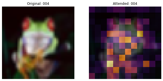
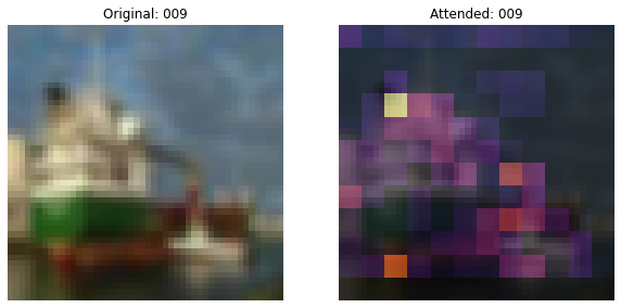
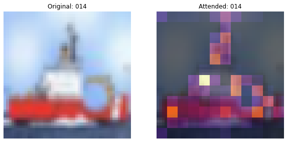
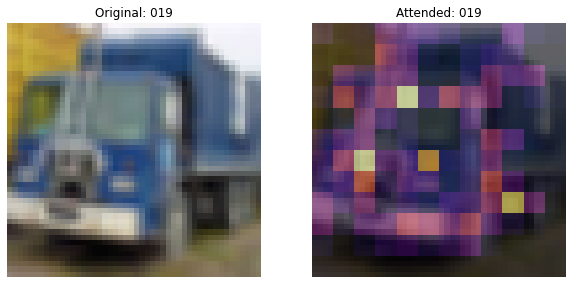
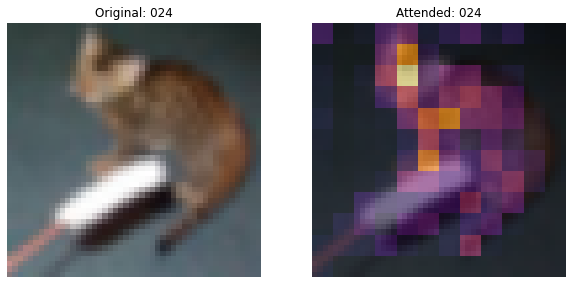
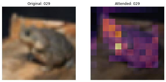
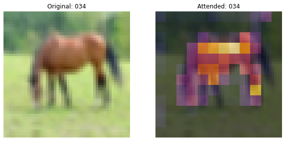
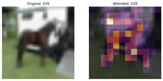
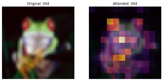
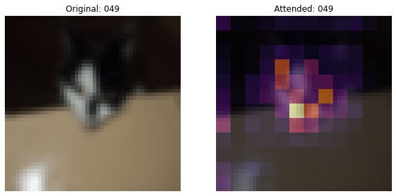
此回调将绘制图像和叠加在图像上的注意力图。
# Taking a batch of test inputs to measure model's progress.
test_images, test_labels = next(iter(test_ds))


class TrainMonitor(keras.callbacks.Callback):
    def __init__(self, epoch_interval=None):
        self.epoch_interval = epoch_interval

    def on_epoch_end(self, epoch, logs=None):
        if self.epoch_interval and epoch % self.epoch_interval == 4:
            test_augmented_images = self.model.preprocessing_model(test_images)
            # Pass through the stem.
            test_x = self.model.stem(test_augmented_images)
            # Pass through the trunk.
            test_x = self.model.trunk(test_x)
            # Pass through the attention pooling block.
            _, test_viz_weights = self.model.attention_pooling(test_x)
            # Reshape the vizualization weights
            num_patches = ops.shape(test_viz_weights)[-1]
            height = width = int(math.sqrt(num_patches))
            test_viz_weights = layers.Reshape((height, width))(test_viz_weights)
            # Take a random image and its attention weights.
            index = np.random.randint(low=0, high=ops.shape(test_augmented_images)[0])
            selected_image = test_augmented_images[index]
            selected_weight = test_viz_weights[index]
            # Plot the images and the overlayed attention map.
            fig, ax = plt.subplots(nrows=1, ncols=2, figsize=(10, 5))
            ax[0].imshow(selected_image)
            ax[0].set_title(f"Original: {epoch:03d}")
            ax[0].axis("off")
            img = ax[1].imshow(selected_image)
            ax[1].imshow(
                selected_weight, cmap="inferno", alpha=0.6, extent=img.get_extent()
            )
            ax[1].set_title(f"Attended: {epoch:03d}")
            ax[1].axis("off")
            plt.axis("off")
            plt.show()
            plt.close()
学习率调度
class WarmUpCosine(keras.optimizers.schedules.LearningRateSchedule):
    def __init__(
        self, learning_rate_base, total_steps, warmup_learning_rate, warmup_steps
    ):
        super().__init__()
        self.learning_rate_base = learning_rate_base
        self.total_steps = total_steps
        self.warmup_learning_rate = warmup_learning_rate
        self.warmup_steps = warmup_steps
        self.pi = np.pi

    def __call__(self, step):
        if self.total_steps < self.warmup_steps:
            raise ValueError("Total_steps must be larger or equal to warmup_steps.")
        cos_annealed_lr = ops.cos(
            self.pi
            * (ops.cast(step, "float32") - self.warmup_steps)
            / float(self.total_steps - self.warmup_steps)
        )
        learning_rate = 0.5 * self.learning_rate_base * (1 + cos_annealed_lr)
        if self.warmup_steps > 0:
            if self.learning_rate_base < self.warmup_learning_rate:
                raise ValueError(
                    "Learning_rate_base must be larger or equal to "
                    "warmup_learning_rate."
                )
            slope = (
                self.learning_rate_base - self.warmup_learning_rate
            ) / self.warmup_steps
            warmup_rate = slope * ops.cast(step, "float32") + self.warmup_learning_rate
            learning_rate = ops.where(
                step < self.warmup_steps, warmup_rate, learning_rate
            )
        return ops.where(
            step > self.total_steps,
            0.0,
            learning_rate,
        )


total_steps = int((len(x_train) / BATCH_SIZE) * EPOCHS)
warmup_epoch_percentage = 0.15
warmup_steps = int(total_steps * warmup_epoch_percentage)
scheduled_lrs = WarmUpCosine(
    learning_rate_base=LEARNING_RATE,
    total_steps=total_steps,
    warmup_learning_rate=0.0,
    warmup_steps=warmup_steps,
)
训练
我们构建模型,编译它,然后训练它。
train_augmentation_model = get_train_augmentation_model()
preprocessing_model = get_preprocessing()
conv_stem = build_convolutional_stem(dimensions=DIMENSIONS)
conv_trunk = Trunk(depth=TRUNK_DEPTH, dimensions=DIMENSIONS, ratio=SE_RATIO)
attention_pooling = AttentionPooling(dimensions=DIMENSIONS, num_classes=NUM_CLASSES)

patch_conv_net = PatchConvNet(
    stem=conv_stem,
    trunk=conv_trunk,
    attention_pooling=attention_pooling,
    train_augmentation_model=train_augmentation_model,
    preprocessing_model=preprocessing_model,
)

# Assemble the callbacks.
train_callbacks = [TrainMonitor(epoch_interval=5)]
# Get the optimizer.
optimizer = keras.optimizers.AdamW(
    learning_rate=scheduled_lrs, weight_decay=WEIGHT_DECAY
)
# Compile and pretrain the model.
patch_conv_net.compile(
    optimizer=optimizer,
    loss=keras.losses.SparseCategoricalCrossentropy(from_logits=True),
    metrics=[
        keras.metrics.SparseCategoricalAccuracy(name="accuracy"),
        keras.metrics.SparseTopKCategoricalAccuracy(5, name="top-5-accuracy"),
    ],
)
history = patch_conv_net.fit(
    train_ds,
    epochs=EPOCHS,
    validation_data=val_ds,
    callbacks=train_callbacks,
)

# Evaluate the model with the test dataset.
loss, acc_top1, acc_top5 = patch_conv_net.evaluate(test_ds)
print(f"Loss: {loss:0.2f}")
print(f"Top 1 test accuracy: {acc_top1*100:0.2f}%")
print(f"Top 5 test accuracy: {acc_top5*100:0.2f}%")
Epoch 1/50
313/313 [==============================] - 14s 27ms/step - loss: 1.9639 - accuracy: 0.2635 - top-5-accuracy: 0.7792 - val_loss: 1.7219 - val_accuracy: 0.3778 - val_top-5-accuracy: 0.8514
Epoch 2/50
313/313 [==============================] - 8s 26ms/step - loss: 1.5475 - accuracy: 0.4214 - top-5-accuracy: 0.9099 - val_loss: 1.4351 - val_accuracy: 0.4592 - val_top-5-accuracy: 0.9298
Epoch 3/50
313/313 [==============================] - 8s 25ms/step - loss: 1.3328 - accuracy: 0.5135 - top-5-accuracy: 0.9368 - val_loss: 1.3763 - val_accuracy: 0.5077 - val_top-5-accuracy: 0.9268
Epoch 4/50
313/313 [==============================] - 8s 25ms/step - loss: 1.1653 - accuracy: 0.5807 - top-5-accuracy: 0.9554 - val_loss: 1.0892 - val_accuracy: 0.6146 - val_top-5-accuracy: 0.9560
Epoch 5/50
313/313 [==============================] - ETA: 0s - loss: 1.0235 - accuracy: 0.6345 - top-5-accuracy: 0.9660
313/313 [==============================] - 8s 25ms/step - loss: 1.0235 - accuracy: 0.6345 - top-5-accuracy: 0.9660 - val_loss: 1.0085 - val_accuracy: 0.6424 - val_top-5-accuracy: 0.9640
Epoch 6/50
313/313 [==============================] - 8s 25ms/step - loss: 0.9190 - accuracy: 0.6729 - top-5-accuracy: 0.9741 - val_loss: 0.9066 - val_accuracy: 0.6850 - val_top-5-accuracy: 0.9751
Epoch 7/50
313/313 [==============================] - 8s 25ms/step - loss: 0.8331 - accuracy: 0.7056 - top-5-accuracy: 0.9783 - val_loss: 0.8844 - val_accuracy: 0.6903 - val_top-5-accuracy: 0.9779
Epoch 8/50
313/313 [==============================] - 8s 25ms/step - loss: 0.7526 - accuracy: 0.7376 - top-5-accuracy: 0.9823 - val_loss: 0.8200 - val_accuracy: 0.7114 - val_top-5-accuracy: 0.9793
Epoch 9/50
313/313 [==============================] - 8s 25ms/step - loss: 0.6853 - accuracy: 0.7636 - top-5-accuracy: 0.9856 - val_loss: 0.7216 - val_accuracy: 0.7584 - val_top-5-accuracy: 0.9823
Epoch 10/50
313/313 [==============================] - ETA: 0s - loss: 0.6260 - accuracy: 0.7849 - top-5-accuracy: 0.9877
313/313 [==============================] - 8s 25ms/step - loss: 0.6260 - accuracy: 0.7849 - top-5-accuracy: 0.9877 - val_loss: 0.6985 - val_accuracy: 0.7624 - val_top-5-accuracy: 0.9847
Epoch 11/50
313/313 [==============================] - 8s 25ms/step - loss: 0.5877 - accuracy: 0.7978 - top-5-accuracy: 0.9897 - val_loss: 0.7357 - val_accuracy: 0.7595 - val_top-5-accuracy: 0.9816
Epoch 12/50
313/313 [==============================] - 8s 25ms/step - loss: 0.5615 - accuracy: 0.8066 - top-5-accuracy: 0.9905 - val_loss: 0.6554 - val_accuracy: 0.7806 - val_top-5-accuracy: 0.9841
Epoch 13/50
313/313 [==============================] - 8s 25ms/step - loss: 0.5287 - accuracy: 0.8174 - top-5-accuracy: 0.9915 - val_loss: 0.5867 - val_accuracy: 0.8051 - val_top-5-accuracy: 0.9869
Epoch 14/50
313/313 [==============================] - 8s 25ms/step - loss: 0.4976 - accuracy: 0.8286 - top-5-accuracy: 0.9921 - val_loss: 0.5707 - val_accuracy: 0.8047 - val_top-5-accuracy: 0.9899
Epoch 15/50
313/313 [==============================] - ETA: 0s - loss: 0.4735 - accuracy: 0.8348 - top-5-accuracy: 0.9939
313/313 [==============================] - 8s 25ms/step - loss: 0.4735 - accuracy: 0.8348 - top-5-accuracy: 0.9939 - val_loss: 0.5945 - val_accuracy: 0.8040 - val_top-5-accuracy: 0.9883
Epoch 16/50
313/313 [==============================] - 8s 25ms/step - loss: 0.4660 - accuracy: 0.8364 - top-5-accuracy: 0.9936 - val_loss: 0.5629 - val_accuracy: 0.8125 - val_top-5-accuracy: 0.9906
Epoch 17/50
313/313 [==============================] - 8s 25ms/step - loss: 0.4416 - accuracy: 0.8462 - top-5-accuracy: 0.9946 - val_loss: 0.5747 - val_accuracy: 0.8013 - val_top-5-accuracy: 0.9888
Epoch 18/50
313/313 [==============================] - 8s 25ms/step - loss: 0.4175 - accuracy: 0.8560 - top-5-accuracy: 0.9949 - val_loss: 0.5672 - val_accuracy: 0.8088 - val_top-5-accuracy: 0.9903
Epoch 19/50
313/313 [==============================] - 8s 25ms/step - loss: 0.3912 - accuracy: 0.8650 - top-5-accuracy: 0.9957 - val_loss: 0.5454 - val_accuracy: 0.8136 - val_top-5-accuracy: 0.9907
Epoch 20/50
311/313 [============================>.] - ETA: 0s - loss: 0.3800 - accuracy: 0.8676 - top-5-accuracy: 0.9956
313/313 [==============================] - 8s 25ms/step - loss: 0.3801 - accuracy: 0.8676 - top-5-accuracy: 0.9956 - val_loss: 0.5274 - val_accuracy: 0.8222 - val_top-5-accuracy: 0.9915
Epoch 21/50
313/313 [==============================] - 8s 25ms/step - loss: 0.3641 - accuracy: 0.8734 - top-5-accuracy: 0.9962 - val_loss: 0.5032 - val_accuracy: 0.8315 - val_top-5-accuracy: 0.9921
Epoch 22/50
313/313 [==============================] - 8s 25ms/step - loss: 0.3474 - accuracy: 0.8805 - top-5-accuracy: 0.9970 - val_loss: 0.5251 - val_accuracy: 0.8302 - val_top-5-accuracy: 0.9917
Epoch 23/50
313/313 [==============================] - 8s 25ms/step - loss: 0.3327 - accuracy: 0.8833 - top-5-accuracy: 0.9976 - val_loss: 0.5158 - val_accuracy: 0.8321 - val_top-5-accuracy: 0.9903
Epoch 24/50
313/313 [==============================] - 8s 25ms/step - loss: 0.3158 - accuracy: 0.8897 - top-5-accuracy: 0.9977 - val_loss: 0.5098 - val_accuracy: 0.8355 - val_top-5-accuracy: 0.9912
Epoch 25/50
312/313 [============================>.] - ETA: 0s - loss: 0.2985 - accuracy: 0.8976 - top-5-accuracy: 0.9976
313/313 [==============================] - 8s 25ms/step - loss: 0.2986 - accuracy: 0.8976 - top-5-accuracy: 0.9976 - val_loss: 0.5302 - val_accuracy: 0.8276 - val_top-5-accuracy: 0.9922
Epoch 26/50
313/313 [==============================] - 8s 25ms/step - loss: 0.2819 - accuracy: 0.9021 - top-5-accuracy: 0.9977 - val_loss: 0.5130 - val_accuracy: 0.8358 - val_top-5-accuracy: 0.9923
Epoch 27/50
313/313 [==============================] - 8s 25ms/step - loss: 0.2696 - accuracy: 0.9065 - top-5-accuracy: 0.9983 - val_loss: 0.5096 - val_accuracy: 0.8389 - val_top-5-accuracy: 0.9926
Epoch 28/50
313/313 [==============================] - 8s 25ms/step - loss: 0.2526 - accuracy: 0.9115 - top-5-accuracy: 0.9983 - val_loss: 0.4988 - val_accuracy: 0.8403 - val_top-5-accuracy: 0.9921
Epoch 29/50
313/313 [==============================] - 8s 25ms/step - loss: 0.2322 - accuracy: 0.9190 - top-5-accuracy: 0.9987 - val_loss: 0.5234 - val_accuracy: 0.8395 - val_top-5-accuracy: 0.9915
Epoch 30/50
313/313 [==============================] - ETA: 0s - loss: 0.2180 - accuracy: 0.9235 - top-5-accuracy: 0.9988
313/313 [==============================] - 8s 26ms/step - loss: 0.2180 - accuracy: 0.9235 - top-5-accuracy: 0.9988 - val_loss: 0.5175 - val_accuracy: 0.8407 - val_top-5-accuracy: 0.9925
Epoch 31/50
313/313 [==============================] - 8s 25ms/step - loss: 0.2108 - accuracy: 0.9267 - top-5-accuracy: 0.9990 - val_loss: 0.5046 - val_accuracy: 0.8476 - val_top-5-accuracy: 0.9937
Epoch 32/50
313/313 [==============================] - 8s 25ms/step - loss: 0.1929 - accuracy: 0.9337 - top-5-accuracy: 0.9991 - val_loss: 0.5096 - val_accuracy: 0.8516 - val_top-5-accuracy: 0.9914
Epoch 33/50
313/313 [==============================] - 8s 25ms/step - loss: 0.1787 - accuracy: 0.9370 - top-5-accuracy: 0.9992 - val_loss: 0.4963 - val_accuracy: 0.8541 - val_top-5-accuracy: 0.9917
Epoch 34/50
313/313 [==============================] - 8s 25ms/step - loss: 0.1653 - accuracy: 0.9428 - top-5-accuracy: 0.9994 - val_loss: 0.5092 - val_accuracy: 0.8547 - val_top-5-accuracy: 0.9921
Epoch 35/50
313/313 [==============================] - ETA: 0s - loss: 0.1544 - accuracy: 0.9464 - top-5-accuracy: 0.9995
313/313 [==============================] - 7s 24ms/step - loss: 0.1544 - accuracy: 0.9464 - top-5-accuracy: 0.9995 - val_loss: 0.5137 - val_accuracy: 0.8513 - val_top-5-accuracy: 0.9928
Epoch 36/50
313/313 [==============================] - 8s 25ms/step - loss: 0.1418 - accuracy: 0.9507 - top-5-accuracy: 0.9997 - val_loss: 0.5267 - val_accuracy: 0.8560 - val_top-5-accuracy: 0.9913
Epoch 37/50
313/313 [==============================] - 8s 25ms/step - loss: 0.1259 - accuracy: 0.9561 - top-5-accuracy: 0.9997 - val_loss: 0.5283 - val_accuracy: 0.8584 - val_top-5-accuracy: 0.9923
Epoch 38/50
313/313 [==============================] - 8s 25ms/step - loss: 0.1166 - accuracy: 0.9599 - top-5-accuracy: 0.9997 - val_loss: 0.5541 - val_accuracy: 0.8549 - val_top-5-accuracy: 0.9919
Epoch 39/50
313/313 [==============================] - 8s 25ms/step - loss: 0.1111 - accuracy: 0.9624 - top-5-accuracy: 0.9997 - val_loss: 0.5543 - val_accuracy: 0.8575 - val_top-5-accuracy: 0.9917
Epoch 40/50
312/313 [============================>.] - ETA: 0s - loss: 0.1017 - accuracy: 0.9653 - top-5-accuracy: 0.9997
313/313 [==============================] - 8s 25ms/step - loss: 0.1016 - accuracy: 0.9653 - top-5-accuracy: 0.9997 - val_loss: 0.5357 - val_accuracy: 0.8614 - val_top-5-accuracy: 0.9923
Epoch 41/50
313/313 [==============================] - 8s 25ms/step - loss: 0.0925 - accuracy: 0.9687 - top-5-accuracy: 0.9998 - val_loss: 0.5248 - val_accuracy: 0.8615 - val_top-5-accuracy: 0.9924
Epoch 42/50
313/313 [==============================] - 8s 25ms/step - loss: 0.0848 - accuracy: 0.9726 - top-5-accuracy: 0.9997 - val_loss: 0.5182 - val_accuracy: 0.8654 - val_top-5-accuracy: 0.9939
Epoch 43/50
313/313 [==============================] - 8s 25ms/step - loss: 0.0823 - accuracy: 0.9724 - top-5-accuracy: 0.9999 - val_loss: 0.5010 - val_accuracy: 0.8679 - val_top-5-accuracy: 0.9931
Epoch 44/50
313/313 [==============================] - 8s 25ms/step - loss: 0.0762 - accuracy: 0.9752 - top-5-accuracy: 0.9998 - val_loss: 0.5088 - val_accuracy: 0.8686 - val_top-5-accuracy: 0.9939
Epoch 45/50
312/313 [============================>.] - ETA: 0s - loss: 0.0752 - accuracy: 0.9763 - top-5-accuracy: 0.9999
313/313 [==============================] - 8s 26ms/step - loss: 0.0752 - accuracy: 0.9764 - top-5-accuracy: 0.9999 - val_loss: 0.4844 - val_accuracy: 0.8679 - val_top-5-accuracy: 0.9938
Epoch 46/50
313/313 [==============================] - 8s 25ms/step - loss: 0.0789 - accuracy: 0.9745 - top-5-accuracy: 0.9997 - val_loss: 0.4774 - val_accuracy: 0.8702 - val_top-5-accuracy: 0.9937
Epoch 47/50
313/313 [==============================] - 8s 25ms/step - loss: 0.0866 - accuracy: 0.9726 - top-5-accuracy: 0.9998 - val_loss: 0.4644 - val_accuracy: 0.8666 - val_top-5-accuracy: 0.9936
Epoch 48/50
313/313 [==============================] - 8s 25ms/step - loss: 0.1000 - accuracy: 0.9697 - top-5-accuracy: 0.9999 - val_loss: 0.4471 - val_accuracy: 0.8636 - val_top-5-accuracy: 0.9933
Epoch 49/50
313/313 [==============================] - 8s 25ms/step - loss: 0.1315 - accuracy: 0.9592 - top-5-accuracy: 0.9997 - val_loss: 0.4411 - val_accuracy: 0.8603 - val_top-5-accuracy: 0.9926
Epoch 50/50
313/313 [==============================] - ETA: 0s - loss: 0.1828 - accuracy: 0.9447 - top-5-accuracy: 0.9995
313/313 [==============================] - 8s 25ms/step - loss: 0.1828 - accuracy: 0.9447 - top-5-accuracy: 0.9995 - val_loss: 0.4614 - val_accuracy: 0.8480 - val_top-5-accuracy: 0.9920
79/79 [==============================] - 1s 8ms/step - loss: 0.4696 - accuracy: 0.8459 - top-5-accuracy: 0.9921
Loss: 0.47
Top 1 test accuracy: 84.59%
Top 5 test accuracy: 99.21%
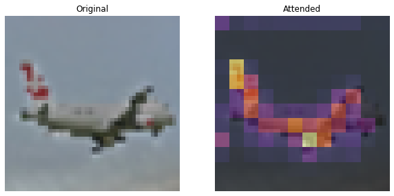
推理
在这里,我们使用训练好的模型来绘制注意力图。
def plot_attention(image):
    """Plots the attention map on top of the image.

    Args:
        image: A numpy image of arbitrary size.
    """
    # Resize the image to a (32, 32) dim.
    image = ops.image.resize(image, (32, 32))
    image = image[np.newaxis, ...]
    test_augmented_images = patch_conv_net.preprocessing_model(image)
    # Pass through the stem.
    test_x = patch_conv_net.stem(test_augmented_images)
    # Pass through the trunk.
    test_x = patch_conv_net.trunk(test_x)
    # Pass through the attention pooling block.
    _, test_viz_weights = patch_conv_net.attention_pooling(test_x)
    test_viz_weights = test_viz_weights[np.newaxis, ...]
    # Reshape the vizualization weights.
    num_patches = ops.shape(test_viz_weights)[-1]
    height = width = int(math.sqrt(num_patches))
    test_viz_weights = layers.Reshape((height, width))(test_viz_weights)
    selected_image = test_augmented_images[0]
    selected_weight = test_viz_weights[0]
    # Plot the images.
    fig, ax = plt.subplots(nrows=1, ncols=2, figsize=(10, 5))
    ax[0].imshow(selected_image)
    ax[0].set_title(f"Original")
    ax[0].axis("off")
    img = ax[1].imshow(selected_image)
    ax[1].imshow(selected_weight, cmap="inferno", alpha=0.6, extent=img.get_extent())
    ax[1].set_title(f"Attended")
    ax[1].axis("off")
    plt.axis("off")
    plt.show()
    plt.close()


url = "http://farm9.staticflickr.com/8017/7140384795_385b1f48df_z.jpg"
image_name = keras.utils.get_file(fname="image.jpg", origin=url)
image = keras.utils.load_img(image_name)
image = keras.utils.img_to_array(image)
plot_attention(image)
结论
与可训练的 CLASS token 和图像 Patch 对应的注意力图有助于解释分类决策。还需要注意的是,注意力图逐渐变得更好。在初始训练阶段,注意力分散在各处,而在后期,它更多地集中在图像的对象上。
非金字塔式卷积网络实现了约 84-85% 的 Top-1 测试准确率。
我要感谢 JarvisLabs.ai 为此项目提供了 GPU 积分。