近似重复图像搜索
作者:Sayak Paul
创建日期 2021/09/10
最后修改日期 2023/08/30

描述: 使用深度学习和局部敏感哈希构建近似重复图像搜索实用程序。
简介
实时(或接近实时)获取相似图像是信息检索系统的一个重要用例。一些利用它的流行产品包括 Pinterest、Google 图片搜索等。在这个示例中,我们将使用局部敏感哈希 (LSH) 和随机投影,基于预训练图像分类器计算的图像表示来构建一个相似图像搜索实用程序。这种搜索引擎也被称为近似重复(或近重复)图像检测器。我们还将研究如何使用TensorRT在 GPU 上优化我们的搜索实用程序的推理性能。
keras.io/examples/vision 下还有其他值得参考的示例:
最后,本示例参考了以下资源并重用了其部分代码:用于相似项目搜索的局部敏感哈希。
请注意,为了优化我们解析器的性能,您应该拥有可用的 GPU 运行时。
设置
!pip install tensorrt
导入
import matplotlib.pyplot as plt
import tensorflow as tf
import tensorrt
import numpy as np
import time

import tensorflow_datasets as tfds

tfds.disable_progress_bar()
加载数据集并创建包含 1,000 张图像的训练集
为了缩短示例运行时间,我们将使用 tf_flowers 数据集(通过TensorFlow Datasets提供)中的 1,000 张图像子集来构建词汇表。
train_ds, validation_ds = tfds.load(
    "tf_flowers", split=["train[:85%]", "train[85%:]"], as_supervised=True
)

IMAGE_SIZE = 224
NUM_IMAGES = 1000

images = []
labels = []

for (image, label) in train_ds.take(NUM_IMAGES):
    image = tf.image.resize(image, (IMAGE_SIZE, IMAGE_SIZE))
    images.append(image.numpy())
    labels.append(label.numpy())

images = np.array(images)
labels = np.array(labels)
加载预训练模型
在本节中,我们加载了一个在 tf_flowers 数据集上训练的图像分类模型。总图像的 85% 用于构建训练集。有关训练的更多详细信息,请参阅此 notebook。
底层模型是 BiT-ResNet(在大迁移 (BiT):通用视觉表示学习中提出)。BiT-ResNet 模型家族以在各种下游任务中提供出色的迁移性能而闻名。
!wget -q https://github.com/sayakpaul/near-dup-parser/releases/download/v0.1.0/flower_model_bit_0.96875.zip
!unzip -qq flower_model_bit_0.96875.zip
bit_model = tf.keras.models.load_model("flower_model_bit_0.96875")
bit_model.count_params()
23510597
创建嵌入模型
给定查询图像检索相似图像,我们首先需要生成所有相关图像的向量表示。我们通过一个嵌入模型来完成此操作,该模型从我们预训练的分类器中提取输出特征并标准化生成的特征向量。
embedding_model = tf.keras.Sequential(
    [
        tf.keras.layers.Input((IMAGE_SIZE, IMAGE_SIZE, 3)),
        tf.keras.layers.Rescaling(scale=1.0 / 255),
        bit_model.layers[1],
        tf.keras.layers.Normalization(mean=0, variance=1),
    ],
    name="embedding_model",
)

embedding_model.summary()
Model: "embedding_model"
_________________________________________________________________
Layer (type)                 Output Shape              Param #
=================================================================
rescaling (Rescaling)        (None, 224, 224, 3)       0
_________________________________________________________________
keras_layer (KerasLayer)     (None, 2048)              23500352
_________________________________________________________________
normalization (Normalization (None, 2048)              0
=================================================================
Total params: 23,500,352
Trainable params: 23,500,352
Non-trainable params: 0
_________________________________________________________________
请注意模型中的归一化层。它用于将表示向量投影到单位球空间。
哈希实用程序
def hash_func(embedding, random_vectors):
    embedding = np.array(embedding)

    # Random projection.
    bools = np.dot(embedding, random_vectors) > 0
    return [bool2int(bool_vec) for bool_vec in bools]


def bool2int(x):
    y = 0
    for i, j in enumerate(x):
        if j:
            y += 1 << i
    return y
从 embedding_model 输出的向量形状是 (2048,),考虑到实际方面(存储、检索性能等),它相当大。因此,需要减少嵌入向量的维度,同时不降低其信息内容。这就是随机投影发挥作用的地方。它基于这样一个原则:如果给定平面上的一组点之间的距离近似保持不变,则该平面的维度可以进一步减小。
在 hash_func() 内部,我们首先减少嵌入向量的维度。然后,我们计算图像的位哈希值以确定它们的哈希桶。具有相同哈希值的图像很可能进入相同的哈希桶。从部署的角度来看,位哈希值存储和操作成本更低。
查询实用程序
Table 类负责构建单个哈希表。哈希表中的每个条目都是我们数据集中图像的缩小嵌入与唯一标识符之间的映射。由于我们的降维技术涉及随机性,因此相似图像可能不会在每次运行时都映射到相同的哈希桶。为了减少这种影响,我们将考虑来自多个表的结果——表的数量和降维是这里的关键超参数。
至关重要的是,在实际应用程序中,您不会自己重新实现局部敏感哈希。相反,您可能会使用以下流行的库之一:
class Table:
    def __init__(self, hash_size, dim):
        self.table = {}
        self.hash_size = hash_size
        self.random_vectors = np.random.randn(hash_size, dim).T

    def add(self, id, vectors, label):
        # Create a unique indentifier.
        entry = {"id_label": str(id) + "_" + str(label)}

        # Compute the hash values.
        hashes = hash_func(vectors, self.random_vectors)

        # Add the hash values to the current table.
        for h in hashes:
            if h in self.table:
                self.table[h].append(entry)
            else:
                self.table[h] = [entry]

    def query(self, vectors):
        # Compute hash value for the query vector.
        hashes = hash_func(vectors, self.random_vectors)
        results = []

        # Loop over the query hashes and determine if they exist in
        # the current table.
        for h in hashes:
            if h in self.table:
                results.extend(self.table[h])
        return results
在下面的 LSH 类中,我们将打包实用程序以拥有多个哈希表。
class LSH:
    def __init__(self, hash_size, dim, num_tables):
        self.num_tables = num_tables
        self.tables = []
        for i in range(self.num_tables):
            self.tables.append(Table(hash_size, dim))

    def add(self, id, vectors, label):
        for table in self.tables:
            table.add(id, vectors, label)

    def query(self, vectors):
        results = []
        for table in self.tables:
            results.extend(table.query(vectors))
        return results
现在我们可以将构建和操作主 LSH 表(许多表的集合)的逻辑封装在一个类中。它有两个方法:
train():负责构建最终的 LSH 表。query():计算给定查询图像的匹配数量并量化相似度分数。
class BuildLSHTable:
    def __init__(
        self,
        prediction_model,
        concrete_function=False,
        hash_size=8,
        dim=2048,
        num_tables=10,
    ):
        self.hash_size = hash_size
        self.dim = dim
        self.num_tables = num_tables
        self.lsh = LSH(self.hash_size, self.dim, self.num_tables)

        self.prediction_model = prediction_model
        self.concrete_function = concrete_function

    def train(self, training_files):
        for id, training_file in enumerate(training_files):
            # Unpack the data.
            image, label = training_file
            if len(image.shape) < 4:
                image = image[None, ...]

            # Compute embeddings and update the LSH tables.
            # More on `self.concrete_function()` later.
            if self.concrete_function:
                features = self.prediction_model(tf.constant(image))[
                    "normalization"
                ].numpy()
            else:
                features = self.prediction_model.predict(image)
            self.lsh.add(id, features, label)

    def query(self, image, verbose=True):
        # Compute the embeddings of the query image and fetch the results.
        if len(image.shape) < 4:
            image = image[None, ...]

        if self.concrete_function:
            features = self.prediction_model(tf.constant(image))[
                "normalization"
            ].numpy()
        else:
            features = self.prediction_model.predict(image)

        results = self.lsh.query(features)
        if verbose:
            print("Matches:", len(results))

        # Calculate Jaccard index to quantify the similarity.
        counts = {}
        for r in results:
            if r["id_label"] in counts:
                counts[r["id_label"]] += 1
            else:
                counts[r["id_label"]] = 1
        for k in counts:
            counts[k] = float(counts[k]) / self.dim
        return counts
创建 LSH 表
实现了我们的辅助实用程序和类之后,我们现在可以构建 LSH 表。由于我们将在优化和未优化嵌入模型之间进行性能基准测试,我们还将预热 GPU 以避免任何不公平的比较。
# Utility to warm up the GPU.
def warmup():
    dummy_sample = tf.ones((1, IMAGE_SIZE, IMAGE_SIZE, 3))
    for _ in range(100):
        _ = embedding_model.predict(dummy_sample)
现在我们可以首先进行 GPU 预热,然后使用 embedding_model 构建主 LSH 表。
warmup()

training_files = zip(images, labels)
lsh_builder = BuildLSHTable(embedding_model)
lsh_builder.train(training_files)
在撰写本文时,在 Tesla T4 GPU 上的墙钟时间为 54.1 秒。此时间可能会因您使用的 GPU 而异。
使用 TensorRT 优化模型
对于基于 NVIDIA 的 GPU,TensorRT 框架可以通过使用各种模型优化技术(如剪枝、常量折叠、层融合等)显著提高推理延迟。这里我们将使用tf.experimental.tensorrt模块来优化我们的嵌入模型。
# First serialize the embedding model as a SavedModel.
embedding_model.save("embedding_model")

# Initialize the conversion parameters.
params = tf.experimental.tensorrt.ConversionParams(
    precision_mode="FP16", maximum_cached_engines=16
)

# Run the conversion.
converter = tf.experimental.tensorrt.Converter(
    input_saved_model_dir="embedding_model", conversion_params=params
)
converter.convert()
converter.save("tensorrt_embedding_model")
WARNING:tensorflow:Compiled the loaded model, but the compiled metrics have yet to be built. `model.compile_metrics` will be empty until you train or evaluate the model.

WARNING:tensorflow:Compiled the loaded model, but the compiled metrics have yet to be built. `model.compile_metrics` will be empty until you train or evaluate the model.

INFO:tensorflow:Assets written to: embedding_model/assets

INFO:tensorflow:Assets written to: embedding_model/assets

INFO:tensorflow:Linked TensorRT version: (0, 0, 0)

INFO:tensorflow:Linked TensorRT version: (0, 0, 0)

INFO:tensorflow:Loaded TensorRT version: (0, 0, 0)

INFO:tensorflow:Loaded TensorRT version: (0, 0, 0)

INFO:tensorflow:Assets written to: tensorrt_embedding_model/assets

INFO:tensorflow:Assets written to: tensorrt_embedding_model/assets
关于 tf.experimental.tensorrt.ConversionParams() 中参数的说明::
precision_mode定义了待转换模型中操作的数值精度。maximum_cached_engines指定了将缓存以处理动态操作(具有未知形状的操作)的 TRT 引擎的最大数量。
要了解更多其他选项,请参阅官方文档。您还可以探索tf.experimental.tensorrt模块提供的不同量化选项。
# Load the converted model.
root = tf.saved_model.load("tensorrt_embedding_model")
trt_model_function = root.signatures["serving_default"]
使用优化模型构建 LSH 表
warmup()

training_files = zip(images, labels)
lsh_builder_trt = BuildLSHTable(trt_model_function, concrete_function=True)
lsh_builder_trt.train(training_files)
请注意墙钟时间的差异,现在是13.1 秒。之前,使用未优化模型时是54.1 秒。
我们可以仔细查看其中一个哈希表,了解它们的表示方式。
idx = 0
for hash, entry in lsh_builder_trt.lsh.tables[0].table.items():
    if idx == 5:
        break
    if len(entry) < 5:
        print(hash, entry)
        idx += 1
145 [{'id_label': '3_4'}, {'id_label': '727_3'}]
5 [{'id_label': '12_4'}]
128 [{'id_label': '30_2'}, {'id_label': '480_2'}]
208 [{'id_label': '34_2'}, {'id_label': '132_2'}, {'id_label': '984_2'}]
188 [{'id_label': '42_0'}, {'id_label': '135_3'}, {'id_label': '436_3'}, {'id_label': '670_3'}]
在验证图像上可视化结果
在本节中,我们将首先编写几个实用函数来可视化相似图像解析过程。然后,我们将对经过优化和未优化模型的查询性能进行基准测试。
首先,我们从验证集中取出 100 张图像进行测试。
validation_images = []
validation_labels = []

for image, label in validation_ds.take(100):
    image = tf.image.resize(image, (224, 224))
    validation_images.append(image.numpy())
    validation_labels.append(label.numpy())

validation_images = np.array(validation_images)
validation_labels = np.array(validation_labels)
validation_images.shape, validation_labels.shape
((100, 224, 224, 3), (100,))
现在我们编写我们的可视化实用程序。
def plot_images(images, labels):
    plt.figure(figsize=(20, 10))
    columns = 5
    for (i, image) in enumerate(images):
        ax = plt.subplot(len(images) // columns + 1, columns, i + 1)
        if i == 0:
            ax.set_title("Query Image\n" + "Label: {}".format(labels[i]))
        else:
            ax.set_title("Similar Image # " + str(i) + "\nLabel: {}".format(labels[i]))
        plt.imshow(image.astype("int"))
        plt.axis("off")


def visualize_lsh(lsh_class):
    idx = np.random.choice(len(validation_images))
    image = validation_images[idx]
    label = validation_labels[idx]
    results = lsh_class.query(image)

    candidates = []
    labels = []
    overlaps = []

    for idx, r in enumerate(sorted(results, key=results.get, reverse=True)):
        if idx == 4:
            break
        image_id, label = r.split("_")[0], r.split("_")[1]
        candidates.append(images[int(image_id)])
        labels.append(label)
        overlaps.append(results[r])

    candidates.insert(0, image)
    labels.insert(0, label)

    plot_images(candidates, labels)
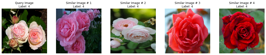
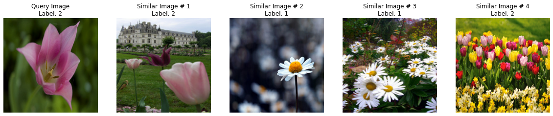
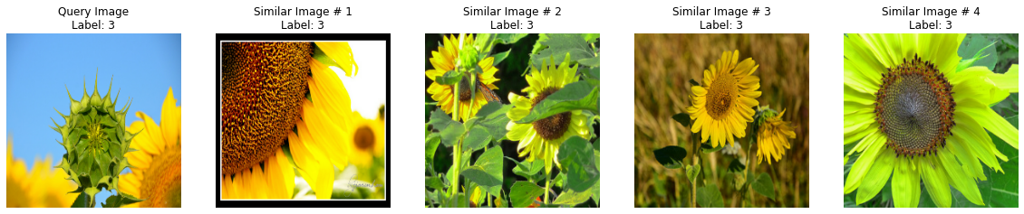
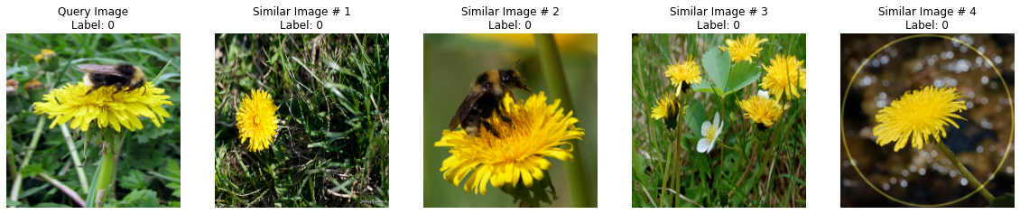
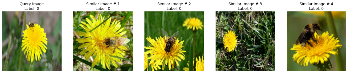
非 TRT 模型
for _ in range(5):
    visualize_lsh(lsh_builder)

visualize_lsh(lsh_builder)
Matches: 507
Matches: 554
Matches: 438
Matches: 370
Matches: 407
Matches: 306
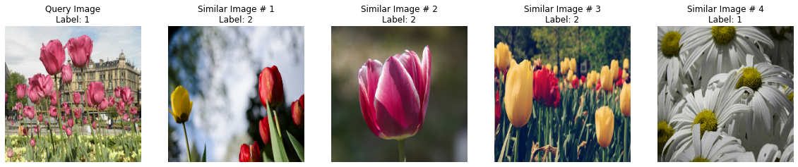
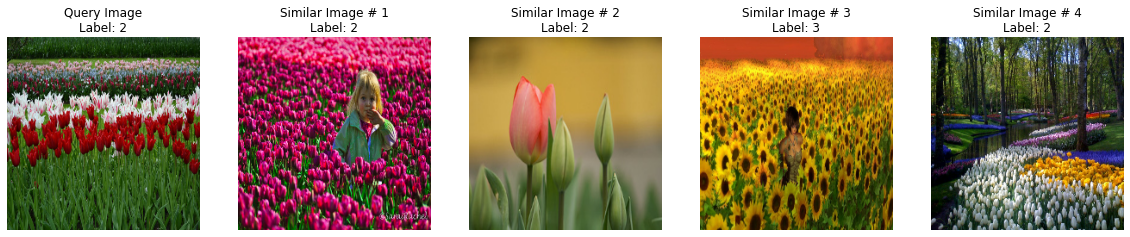
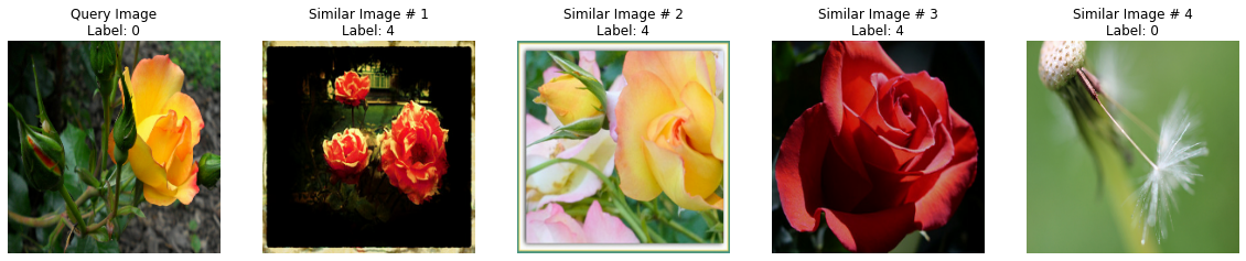
TRT 模型
for _ in range(5):
    visualize_lsh(lsh_builder_trt)
Matches: 458
Matches: 181
Matches: 280
Matches: 280
Matches: 503
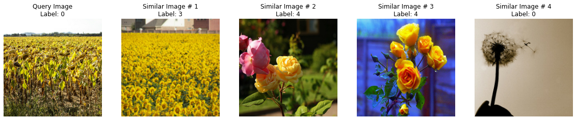

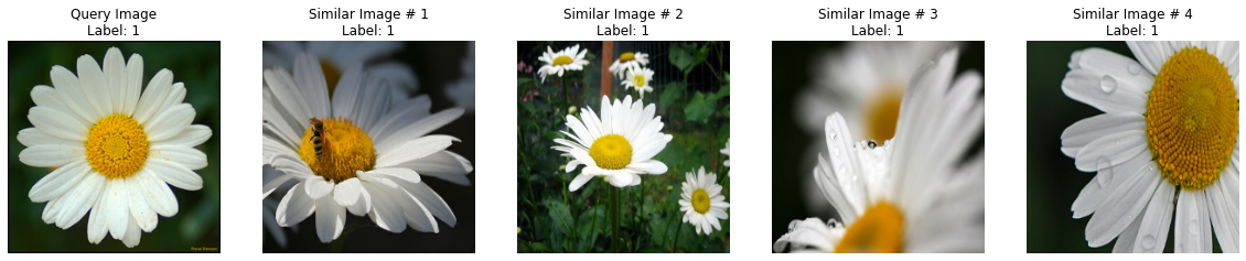
您可能已经注意到,存在一些不正确的结果。这可以通过以下几种方式进行缓解:
- 用于生成初始嵌入的更好模型,特别是针对噪声样本。我们可以使用ArcFace、监督对比学习等技术,这些技术隐式地鼓励更好地学习用于检索目的的表示。
- 表的数量和降维之间的权衡至关重要,它有助于为您的应用程序设置所需的召回率。
基准测试查询性能
def benchmark(lsh_class):
    warmup()

    start_time = time.time()
    for _ in range(1000):
        image = np.ones((1, 224, 224, 3)).astype("float32")
        _ = lsh_class.query(image, verbose=False)
    end_time = time.time() - start_time
    print(f"Time taken: {end_time:.3f}")


benchmark(lsh_builder)

benchmark(lsh_builder_trt)
Time taken: 54.359
Time taken: 13.963
我们可以立即注意到两个模型的查询性能之间存在显著差异。
最后说明
在这个例子中,我们探索了 NVIDIA 的 TensorRT 框架来优化我们的模型。它最适合基于 GPU 的推理服务器。还有其他此类框架可满足不同的硬件平台需求:
- TensorFlow Lite 适用于移动和边缘设备。
- ONNX 适用于基于商品 CPU 的服务器。
- Apache TVM,用于涵盖各种平台的机器学习模型编译器。
以下是一些您可能想查看的资源,以了解更多关于基于向量相似性搜索的应用程序: