► 代码示例 / 计算机视觉 / 使用 BigTransfer (BiT) 进行图像分类

使用 BigTransfer (BiT) 进行图像分类

作者： Sayan Nath
创建日期 2021/09/24
最后修改 2024/01/03
描述： BigTransfer (BiT) 最先进的图像分类迁移学习方法。

ⓘ 此示例使用 Keras 3

引言

BigTransfer (也称为 BiT) 是一种最先进的图像分类迁移学习方法。预训练表示的迁移提高了样本效率，并简化了训练用于视觉的深度神经网络时的超参数调优。BiT 重新审视了在大型有监督数据集上进行预训练并在目标任务上微调模型的范式。随着预训练数据量的增加，适当选择归一化层和扩展架构容量的重要性。

BigTransfer(BiT) 在公共数据集上进行训练，并提供 TF2、Jax 和 Pytorch 代码。这可以帮助任何人在其感兴趣的任务上达到最先进的性能，即使每类只有少量标注图像。

您可以在 TFHub 中找到在 ImageNet 和 ImageNet-21k 上预训练的 BiT 模型，它们是 TensorFlow2 SavedModels，您可以轻松地将其用作 Keras 层。模型尺寸多样，从标准的 ResNet50 到 ResNet152x4 (152 层深，比典型的 ResNet50 宽 4 倍)，以满足计算和内存预算较大但对精度要求更高的用户。

图：x 轴表示每类使用的图像数量，范围从 1 到整个数据集。在左侧的图中，上方蓝色曲线是我们的 BiT-L 模型，而下方曲线是在 ImageNet (ILSVRC-2012) 上预训练的 ResNet-50。

设置

import os
os.environ["KERAS_BACKEND"] = "tensorflow"
import numpy as np
import pandas as pd
import matplotlib.pyplot as plt

import keras
from keras import ops
import tensorflow as tf
import tensorflow_hub as hub
import tensorflow_datasets as tfds

tfds.disable_progress_bar()

SEEDS = 42

keras.utils.set_random_seed(SEEDS)

收集花卉数据集

train_ds, validation_ds = tfds.load(
    "tf_flowers",
    split=["train[:85%]", "train[85%:]"],
    as_supervised=True,
)

[1mDownloading and preparing dataset 218.21 MiB (download: 218.21 MiB, generated: 221.83 MiB, total: 440.05 MiB) to ~/tensorflow_datasets/tf_flowers/3.0.1...[0m
[1mDataset tf_flowers downloaded and prepared to ~/tensorflow_datasets/tf_flowers/3.0.1. Subsequent calls will reuse this data.[0m

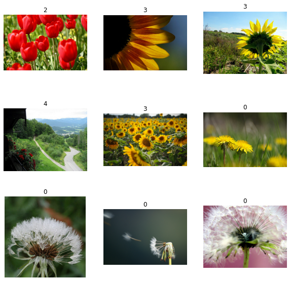
可视化数据集

plt.figure(figsize=(10, 10))
for i, (image, label) in enumerate(train_ds.take(9)):
    ax = plt.subplot(3, 3, i + 1)
    plt.imshow(image)
    plt.title(int(label))
    plt.axis("off")

png

定义超参数

RESIZE_TO = 384
CROP_TO = 224
BATCH_SIZE = 64
STEPS_PER_EPOCH = 10
AUTO = tf.data.AUTOTUNE  # optimise the pipeline performance
NUM_CLASSES = 5  # number of classes
SCHEDULE_LENGTH = (
    500  # we will train on lower resolution images and will still attain good results
)
SCHEDULE_BOUNDARIES = [
    200,
    300,
    400,
]  # more the dataset size the schedule length increase

SCHEDULE_LENGTH 和 SCHEDULE_BOUNDARIES 等超参数是根据经验结果确定的。该方法已在原始论文和他们的Google AI 博客文章中进行了解释。

SCHEDULE_LENGTH 也决定了是否使用MixUp 数据增强。您还可以在Keras 代码示例中找到一个简单的 MixUp 实现。

定义预处理辅助函数

SCHEDULE_LENGTH = SCHEDULE_LENGTH * 512 / BATCH_SIZE

random_flip = keras.layers.RandomFlip("horizontal")
random_crop = keras.layers.RandomCrop(CROP_TO, CROP_TO)

def preprocess_train(image, label):
    image = random_flip(image)
    image = ops.image.resize(image, (RESIZE_TO, RESIZE_TO))
    image = random_crop(image)
    image = image / 255.0
    return (image, label)


def preprocess_test(image, label):
    image = ops.image.resize(image, (RESIZE_TO, RESIZE_TO))
    image = ops.cast(image, dtype="float32")
    image = image / 255.0
    return (image, label)


DATASET_NUM_TRAIN_EXAMPLES = train_ds.cardinality().numpy()

repeat_count = int(
    SCHEDULE_LENGTH * BATCH_SIZE / DATASET_NUM_TRAIN_EXAMPLES * STEPS_PER_EPOCH
)
repeat_count += 50 + 1  # To ensure at least there are 50 epochs of training

定义数据管道

# Training pipeline
pipeline_train = (
    train_ds.shuffle(10000)
    .repeat(repeat_count)  # Repeat dataset_size / num_steps
    .map(preprocess_train, num_parallel_calls=AUTO)
    .batch(BATCH_SIZE)
    .prefetch(AUTO)
)

# Validation pipeline
pipeline_validation = (
    validation_ds.map(preprocess_test, num_parallel_calls=AUTO)
    .batch(BATCH_SIZE)
    .prefetch(AUTO)
)

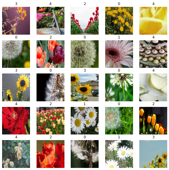
可视化训练样本

image_batch, label_batch = next(iter(pipeline_train))

plt.figure(figsize=(10, 10))
for n in range(25):
    ax = plt.subplot(5, 5, n + 1)
    plt.imshow(image_batch[n])
    plt.title(label_batch[n].numpy())
    plt.axis("off")

png

将预训练的 TF-Hub 模型加载到 KerasLayer 中

bit_model_url = "https://tfhub.dev/google/bit/m-r50x1/1"
bit_module = hub.load(bit_model_url)

创建 BigTransfer (BiT) 模型

创建新模型，我们需要

ตัด bỏ BiT 模型的原始头部。这会得到“pre-logits”输出。如果我们使用“特征提取器”模型（即所有位于名为 feature_vectors 的子目录中的模型），则无需执行此操作，因为这些模型的头部已被 cắt bỏ。
添加一个新头部，其输出数量等于我们新任务的类别数量。请注意，将头部初始化为全零很重要。

class MyBiTModel(keras.Model):
    def __init__(self, num_classes, module, **kwargs):
        super().__init__(**kwargs)

        self.num_classes = num_classes
        self.head = keras.layers.Dense(num_classes, kernel_initializer="zeros")
        self.bit_model = module

    def call(self, images):
        bit_embedding = self.bit_model(images)
        return self.head(bit_embedding)


model = MyBiTModel(num_classes=NUM_CLASSES, module=bit_module)

定义优化器和损失函数

learning_rate = 0.003 * BATCH_SIZE / 512

# Decay learning rate by a factor of 10 at SCHEDULE_BOUNDARIES.
lr_schedule = keras.optimizers.schedules.PiecewiseConstantDecay(
    boundaries=SCHEDULE_BOUNDARIES,
    values=[
        learning_rate,
        learning_rate * 0.1,
        learning_rate * 0.01,
        learning_rate * 0.001,
    ],
)
optimizer = keras.optimizers.SGD(learning_rate=lr_schedule, momentum=0.9)

loss_fn = keras.losses.SparseCategoricalCrossentropy(from_logits=True)

编译模型

model.compile(optimizer=optimizer, loss=loss_fn, metrics=["accuracy"])

设置回调

train_callbacks = [
    keras.callbacks.EarlyStopping(
        monitor="val_accuracy", patience=2, restore_best_weights=True
    )
]

训练模型

history = model.fit(
    pipeline_train,
    batch_size=BATCH_SIZE,
    epochs=int(SCHEDULE_LENGTH / STEPS_PER_EPOCH),
    steps_per_epoch=STEPS_PER_EPOCH,
    validation_data=pipeline_validation,
    callbacks=train_callbacks,
)

Epoch 1/400
10/10 [==============================] - 18s 852ms/step - loss: 0.7465 - accuracy: 0.7891 - val_loss: 0.1865 - val_accuracy: 0.9582
Epoch 2/400
10/10 [==============================] - 5s 529ms/step - loss: 0.1389 - accuracy: 0.9578 - val_loss: 0.1075 - val_accuracy: 0.9727
Epoch 3/400
10/10 [==============================] - 5s 520ms/step - loss: 0.1720 - accuracy: 0.9391 - val_loss: 0.0858 - val_accuracy: 0.9727
Epoch 4/400
10/10 [==============================] - 5s 525ms/step - loss: 0.1211 - accuracy: 0.9516 - val_loss: 0.0833 - val_accuracy: 0.9691

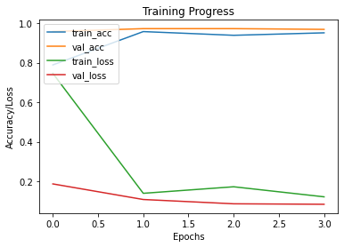
绘制训练和验证指标

def plot_hist(hist):
    plt.plot(hist.history["accuracy"])
    plt.plot(hist.history["val_accuracy"])
    plt.plot(hist.history["loss"])
    plt.plot(hist.history["val_loss"])
    plt.title("Training Progress")
    plt.ylabel("Accuracy/Loss")
    plt.xlabel("Epochs")
    plt.legend(["train_acc", "val_acc", "train_loss", "val_loss"], loc="upper left")
    plt.show()


plot_hist(history)

png

评估模型

accuracy = model.evaluate(pipeline_validation)[1] * 100
print("Accuracy: {:.2f}%".format(accuracy))

9/9 [==============================] - 3s 364ms/step - loss: 0.1075 - accuracy: 0.9727
Accuracy: 97.27%

结论

BiT 在令人惊讶的广泛数据范围内表现出色——从每类 1 个示例到总共 100 万个示例。BiT 在 ILSVRC-2012 上达到了 87.5% 的 top-1 准确率，在 CIFAR-10 上达到了 99.4%，在 19 个任务的视觉任务适应基准 (VTAB) 上达到了 76.3%。在小型数据集上，BiT 在 ILSVRC-2012 上每类 10 个示例时达到了 76.8%，在 CIFAR-10 上每类 10 个示例时达到了 97.0%。